Radiative Cooling of Gravitationally Collapsing Molecular Cloud

Colliding flows and the birth of stars

Caption_right

Star-forming region S106 (captured by the Hubble Space Telescope)

The birth of stars is one of the most captivating processes in astrophysics, yet the journey from a vast, diffuse gas cloud to a brilliant new star is anything but simple. At the heart of this transformation lies the gravitational collapse of molecular clouds—cold, dense pockets of interstellar gas that serve as stellar nurseries. But what sets this collapse in motion? The answer probably lies in colliding flows, where turbulent gas streams crash into one another, compressing the material and setting the stage for star formation. Since molecular clouds are significantly denser than their surroundings, compression is inevitable. However, the real puzzle is identifying the forces that drive this compression and understanding how they shape the evolution of these structures.

The power of shock waves

Within molecular clouds, which are cold and compact parts of interstellar space, multiple processes can trigger the creation of shock waves. These processes could be the collision of diverse gas streams or the movement of the cloud itself through the interstellar medium. When these shock waves travel through the gas in a molecular cloud, they condense the gas, increasing its density. The condensation brought about by shock waves can be a key factor for setting in motion the process of gravitational collapse, ultimately leading to the formation of stars. Through this gas compression, shock waves enhance the density of specific regions within the cloud. These denser areas are more apt to overcome the internal gas pressure and start collapsing under the influence of gravity.

Self-similarity: patterns in the chaos

Caption_left

Murakami et al. (2004)

Despite the seemingly chaotic nature of collapsing clouds, a fascinating pattern emerges—one rooted in self-similarity. In physics, self-similarity means that a system looks the same at different scales, following a predictable mathematical pattern. For example, you would probably be familiar with the Larson-Penston (LP) solution (Larson 1969; Penston 1969) which utilizes the continuity and momentum conservation equation to give a self-similar solution for the gravitational collapse of an isothermal gaseous sphere.

The behavior of x (distance or radius) and t (time) in these self-similar solutions could be such that the radius and density are related by a power-law expression that remains constant as the collapse progresses. This means that if you were to plot the density profile of the cloud at different times, the shape of the profile would remain the same, but the scale would change according to a power-law relationship with time.

Planar geometry

Caption_right

Plane-parallel geometry

In this project, the approach is to utilize a plane-parallel geometry, where variations in physical properties solely arise along the x-axis and are assumed uniform along the y and z axes. Thus, in a system or flow displaying self-similar traits in this plane-parallel geometry, fluid properties such as velocity, temperature, and density follow a consistent pattern of change regardless of the scale of observation.

So we will have:

• $v=v_x,\rho ={\rho }_x$
• $\frac{d}{dy}=\frac{d}{dz}=0$

Radiative cooling

A key assumption that we made for this particular problem is that radiative losses balance out compressional heating, maintaining a relatively low temperature for the contracting gas cloud. In simpler terms, as the gas becomes compressed during collapse, the increased internal energy can escape through radiation, causing the gas to heat up less efficiently compared to what one would anticipate for gas undergoing adiabatic compression.

Objectives

The objective here is to present a self-similar solution that considers two physical phenomena: self-gravity and radiative cooling.

• We address the complete set of hydrodynamic equations,
• Introduce a cooling term into the energy equation to account for heat loss, and search for self-similar solutions.

The physical system

The compressible Navier-Stokes equations with cooling are formulated as follows:

$$\frac{\partial \rho }{\partial t}+\nabla \cdot (\rho \mathbf{u})=0$$ $$\frac{\partial \rho \mathbf{u}}{\partial t}+\nabla \cdot (\rho \mathbf{uu})=-\nabla P-\rho \nabla \varphi$$ $$\Delta \varphi =4\pi G\rho$$ $$\frac{\partial \rho (ϵ+\frac{u^2}{2})}{\partial t}+\nabla \cdot \left[\rho \left(ϵ+\frac{u^2}{2}\right)\mathbf{u}\right]=-\nabla \cdot (P\mathbf{u})-\rho \mathbf{u}\cdot \nabla \varphi -\Lambda$$

where t is time, u is the velocity vector, φ is the gravitational potential, G is the gravitational constant, $ϵ$ is the specific internal energy and Λ is the volumic cooling rate. The heat interchange encompasses both heating and cooling, though our focus is solely on situations where cooling surpasses heating. As a result, the combined effect of these two is negative here. The behavior of the gas adheres to the principles of the ideal gas law.

$$\frac{k_B}{\mu m_p}T=\frac{P}{\rho }=(\gamma -1)ϵ$$

where $k_B$ is the Boltzmann constant, µ is the mean particle (molecular) weight, $m_P$ is the proton mass, $\gamma$ is the specific heat ratio, and T is the temperature.

We parameterize the cooling function as:

$$\Lambda ={\Lambda }_0{\rho }^m{T}^n,{\Lambda }_0\in {\mathbb{R}}^{+}$$

For the values of m and n:

• Depending on the cooling mechanism, we can have m = 1 or 2:
  • m = 2 for collisional cooling
  • m = 1 for thermal radiation
• Since it’s a nonlinear steep dependence on temperature, we can approximate with a power law that has n larger than 1.

Next, we define the mass per unit area as:

$$\Sigma ={\int }_0^x\rho dx$$

From Gauss’s law for gravity:

$$\int \text{g}\cdot \text{n}=2g=-4\pi G2\Sigma$$ $$\to g=-2\pi G2\Sigma =-\nabla \varphi$$

Thus, in the x dimension:

$$\frac{\partial \varphi }{\partial x}=2\pi G2\Sigma$$

Now, the one-dimensional system for planar symmetry can be written as follows:

$$\frac{\partial \rho }{\partial t}+\frac{\partial (\rho u)}{\partial x}=0\text{\hspace{1em}(1)}$$ $$\frac{\partial u}{\partial t}+u\frac{\partial u}{\partial x}=-\frac{1}{\rho }\frac{\partial P}{\partial x}-4\pi G\Sigma \text{\hspace{1em}(2)}$$ $$\Sigma ={\int }_0^x\rho dx\text{\hspace{1em}(3)}$$ $$\rho \left(\frac{\partial ϵ}{\partial t}+u\frac{\partial ϵ}{\partial x}\right)=-P\frac{\partial u}{\partial x}-{\Lambda }_0{\rho }^m{T}^n\text{\hspace{1em}(4)}$$

Self-similar equations

We will use the above equations and the ideal gas law, along with the following group transformation:

$$x=\lambda \hat{x},t={\lambda }^a\hat{t},u={\lambda }^b\hat{u},T={\lambda }^c\hat{T},\rho ={\lambda }^d\hat{\rho },\varphi ={\lambda }^e\hat{\varphi }$$

Here, the symbols with hats represent the scaled physical quantities in relation to the unscaled parent system by the scaling factor $\lambda$. To ensures symmetry and equivalence of structure between the transformed system and the original system for self-similarity to exist, the constants a, b, c, d, and e must satisfy the following conditions:

$$1-a=b=\frac{c}{2}=1+\frac{d}{2}=\frac{e}{2}=\frac{3-2m}{5-2m-2n}\text{\hspace{1em}(5)}$$

The following similarity Ansatz (inspired by Murakami et al. 2004) would allow us to eliminate the temporal dependence from the one-dimensional system equations. Basically, all the scales of the physical quantities are uniquely determined as a function of time only:

$$x=A|t{|}^{1/a}\xi \text{\hspace{1em}(6)}$$ $$u=\frac{A}{a}|t{|}^{b/a}\nu (\xi )\text{\hspace{1em}(7)}$$ $$T=\frac{A^2}{a^2}\frac{\mu m_p}{k_B}|t{|}^{c/a}\tau (\xi )\text{\hspace{1em}(8)}$$ $$\rho =B|t{|}^{-2}g(\xi )\text{\hspace{1em}(9)}$$ $$\frac{\partial \varphi }{\partial x}=2\pi G2\Sigma =4\pi GAB|t{|}^{(e-1)/a}\sigma (\xi )\text{\hspace{1em}(10)}$$ $$\Sigma ={\Sigma }_0+{\int }_0^x\rho dx=AB|t{|}^{1/a-2}\sigma (\xi )\text{\hspace{1em}(11)}$$ $$\sigma (\xi )={\sigma }_0+{\int }_0^{\xi }g(\xi )d\xi \text{\hspace{1em}(12)}$$

Here, A and B are positive constants that establish the scales of the radius and density. It’s important to observe that the relationship d/a = -2 is applied to the density equation’s similarity approach, and this remains valid regardless of the specific values of m and n.

From the above similarity, the equations governing mass conservation, momentum conservation, and energy conservation are simplified into the subsequent sets of ordinary differential equations:

$$(\nu \mp \xi )g^{\prime }+({\nu }^{\prime }\pm d)g=0\text{\hspace{1em}(13)}$$ $$\pm b\nu +(\nu \mp \xi ){\nu }^{\prime }+\frac{(g\tau {)}^{\prime }}{g}+K_1\sigma =0\text{\hspace{1em}(14)}$$ $$\frac{\pm c\tau +(\nu \mp \xi ){\tau }^{\prime }}{\gamma -1}+\tau {\nu }^{\prime }+K_2{g}^{m-1}{\tau }^n=0\text{\hspace{1em}(15)}$$

where the prime denotes the derivative with respect to ξ and the plus and minus signs correspond to t>0 and t<0. You may have noticed that we had four equations in the system, where the third equation is Poisson’s equation for gravity. But this equation is automatically satisfied in the above step, so we don’t need to include its reduced form here. These three ODEs are a second-order ODE system for g, τ and v.

Apparently, the system above is characterized by two dimensionless parameters $K_1$ and $K_2$:

$$K_1=4\pi a^{2}GB$$ $$K_2={\Lambda }_{0}a{B}^{m-1}{\left(\frac{A}{a}\right)}^{2(n-1)}{\left(\frac{\mu m_p}{k_B}\right)}^n$$

Additionally, from the mass conservation law:

$$\frac{\partial \Sigma }{\partial t}=-\rho u\text{\hspace{1em}(16)}$$ $$\sigma =\frac{g(\xi \mp \nu )}{1-2a}\text{\hspace{1em}(17)}$$

Asymptotic behaviors

An analytical solution is not available for this nonlinear system, except for a single trivial solution when t < 0. However, we can deduce asymptotic solutions under specific constraints and utilize numerical integration to acquire full solutions. We use the terminology introduced by Whitworth & Summers (1985) and identify three regimes: the early interior path (t < 0 and ξ is small), the exterior path (ξ is large), and the late path (t > 0 and ξ is small).

For now, I’ve only managed to investigate the first regime - the early interior path (t<0, ξ <<1).

Early interior path

The time interval t < 0 corresponds to the period preceding the formation of a mass singularity at the core of the collapsing area. During this phase, the central region exhibits a homologous collapse with a flat density and temperature profile. We assume the following polynomial series:

$$g=1+g_1\xi +g_2{\xi }^2+\mathcal{O}({\xi }^3)\text{\hspace{1em}(18)}$$ $$\nu ={\nu }_0+{\nu }_1\xi +{\nu }_2{\xi }^2+{\nu }_3{\xi }^3+\mathcal{O}({\xi }^4)\text{\hspace{1em}(19)}$$ $$\tau =1+{\tau }_1\xi +{\tau }_2{\xi }^2+\mathcal{O}({\xi }^3)\text{\hspace{1em}(20)}$$

As A and B are adjustable parameters, we have the flexibility to opt for a scaling that ensures the leading term of both g and τ is set to one. The physical boundary conditions is as follows:

$$g^{\prime }(0)=0,\nu (0)=0,{\tau }^{\prime }(0)=0$$

This suggests that there is no singularity present at the origin, no density and temperature gradient. When we substitute these values into the equations, we readily determine that $g_1={\nu }_0={\nu }_2={\tau }_1=0$. Essentially, due to symmetry considerations, all odd-order terms of g and τ, as well as even-order terms of v, must become null. This simplifies the polynomial series to:

$$g=1+g_2{\xi }^2,\nu ={\nu }_1\xi +{\nu }_3{\xi }^3,\tau =1+{\tau }_2{\xi }^2\text{\hspace{1em}(21)}$$

Inserting into the ODE system, we can get:

$${\nu }_1=d=\frac{4n-4}{5-2m-2n}\text{\hspace{1em}(22)}$$ $$2g_2({\nu }_1+1)+3{\nu }_3=0\text{\hspace{1em}(23)}$$ $$g_2+{\tau }_2=-\frac{{\nu }_1^2}{4}-\frac{K_1}{2}\text{\hspace{1em}(24)}$$ $${\tau }_2=\frac{11a^2}{6}-\frac{11a}{6}-\frac{1}{3}(K_1-1)\text{\hspace{1em}(25)}$$ $$g_2=\left(-\frac{v_1^2}{4}-\frac{K_1}{2}\right)\frac{2\frac{{\nu }_1+1}{\gamma -1}+(n-1)K_2}{2\gamma \frac{{\nu }_1+1}{\gamma -1}+(n-m)K_2}\text{\hspace{1em}(26)}$$ $$K_2=\frac{c}{\gamma -1}-d\text{\hspace{1em}(27)}$$

It’s apparent that $K_1$ plays a crucial role in determining both the magnitude and sign of $g_2$. In our polynomial series, setting ${\tau }_0$ to a value of 1 is essentially the same as fixing the value of $K_2$. Altering ${\tau }_0$ and $K_2$ induces a rescaling effect on the system, which results in precisely the same solution when reverted back to physical units.

From the constraints above, it is apparent that for $g_2$ and ${\tau }_2$ to be equal to 0, we must have:

$$K_1=K_0=-\frac{{\nu }_1^2}{2}$$

The effective polytropic index can be obtained by substituting the asymptotic values into the equation that represents the effective equation of state (EOS),

$$P\propto {\rho }^{\Gamma }\text{\hspace{1em}(28)}$$

leading to:

$${\tau }_2=g_2({\Gamma }_i-1)\text{\hspace{1em}(29)}$$

Using the constraints above again, we have:

$${\Gamma }_i=\frac{g_2+{\tau }_2}{g_2}=\frac{2\gamma (d+1)+(n-m)(c-(\gamma -1)d)}{2(d+1)+(n-1)(c-(\gamma -1)d)}\text{\hspace{1em}(30)}$$

Apparently, ${\Gamma }_i$ is a weighted mean between $\gamma$ and $(n-m)/(n-1)$.

Sonic point

Studying a singular point is of utmost importance as it provides significant insights into the behavior of the system. However, with the complexity due to the energy conservation equation within our system, analyzing them analytically is challenging.

By expressing the set of ODEs as linear combinations of their derivatives, we can derive:

$$g^{\prime }=\frac{{\Delta }_1}{\Delta },{\nu }^{\prime }=\frac{{\Delta }_2}{\Delta },{\tau }^{\prime }=\frac{{\Delta }_3}{\Delta }\text{\hspace{1em}(31)}$$

where:

$$\Delta =(\nu \mp \xi )\left[\tau -\frac{(\nu \mp \xi {)}^2-\tau }{\gamma -1}\right]$$ $${\Delta }_1=-\frac{g}{\gamma -1}\left[\mp c\tau \mp \frac{K_1}{1-2a}g(\nu \mp \xi {)}^2\pm b\nu (\nu \mp \xi )\mp d(\nu \mp \xi {)}^2\right]+K_2{g}^m{\tau }^n\mp dg\tau$$ $${\Delta }_2=\frac{\nu \mp \xi }{\gamma -1}\left[\mp c\tau \mp \frac{K_1}{1-2a}g(\nu \mp \xi {)}^2\pm b\nu (\nu \mp \xi )\mp d\tau \right]-(\nu \mp \xi )K_2{g}^{m-1}{\tau }^n$$ $${\Delta }_3=[(\nu \mp \xi {)}^2-\tau ](K_2{g}^{m-1}{\tau }^n\pm \frac{c\tau }{\gamma -1})\pm \tau \frac{K_1}{1-2a}g(\nu \mp \xi {)}^2\mp b\nu \tau (\nu \mp \xi )\pm d{\tau }^2$$

whew yeah that’s a lot…

So in order for the solutions with t<0 to transition smoothly through the sonic surface, it is necessary for both conditions,

$$\Delta ={\Delta }_2=0\text{\hspace{1em}(32)}$$

to be met simultaneously at the sonic point, which is where the solution intersects the sonic surface.

Two distinct types of solutions can smoothly pass through the sonic point.

• The first type is a trivial case with $K_1=K_0=-\frac{{\nu }_1^2}{2}$, resulting in constant density and temperature. This leads to a linear velocity profile.
• The second valid value of $K_1$ needs to be determined through numerical integration, using the shooting method towards the sonic point. Essentially, we solve the above problem by reducing it to an initial value problem. We find solutions for different initial values of $K_1$ until we find the solution that also satisfies the sonic surface conditions mentioned above.

Results

Trivial solution

When $K_1=K_0=-\frac{{\nu }_1^2}{2}$, a trivial solution is pretty easy to find:

$$g(\xi )=1,\nu (\xi )=d\xi ,\tau (\xi )=1.\text{\hspace{1em}(33)}$$

This solution characterizes the homologous collapse of a flat structure that stretches infinitely and is applicable solely for t < 0.

Physical solution

We employ numerical methods to solve the system, initializing integration at ξ values considerably small and at times t < 0. By utilizing the shooting method, we determine the appropriate value of K1 that permits the existence of a continuous solution. Subsequently, the negative solution is extrapolated to very large ξ values. In the below figure, we present illustrative profiles for two chosen pairs of m and n.

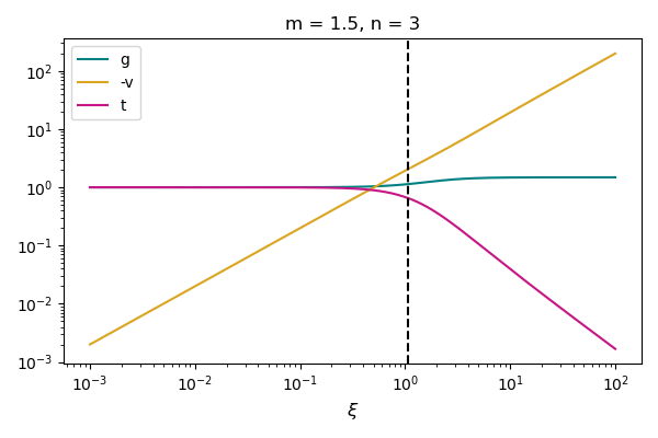
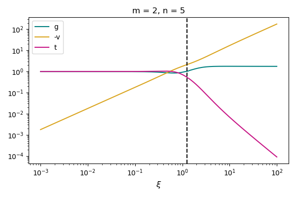
Self-similar solution for two cases: (m, n) = (1.5, 3), (2, 5) from top to bottom. The dimensionless density, velocity and temperature are shown in blue, orange and green respectively. The dashed line shows the sonic point.

From the velocity profile (yellow line), we can see that the compression is faster than the sonic velocity; thus, we have a supersonic collapse.

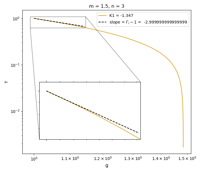
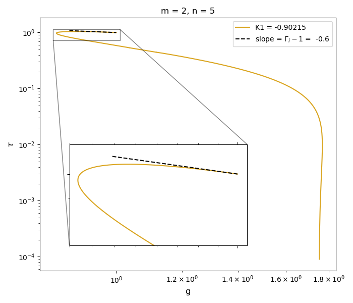
Density-temperature diagram for two cases: (m, n) = (1.5, 3), (2, 5) from top to bottom. The dashed line shows the slope from the asymptotic solution.

We recall that ${\tau }_2=g_2({\Gamma }_i-1)$, where ${\Gamma }_i-1$ is shown on the figures above. Obviously, both the numerical and asymptotic solutions give the same slope values.