So far, we’ve looked at the zero-dimensional energy balance model (EBM), which treats Earth as a single, uniform entity. But the real climate system isn’t that simple—especially when it comes to latitude. Solar radiation varies significantly from the equator to the poles, and factors like ice feedbacks play a major role in shaping regional climates. To capture these variations, we need to add a spatial dimension to our model.

The One-Dimensional Energy Balance Model

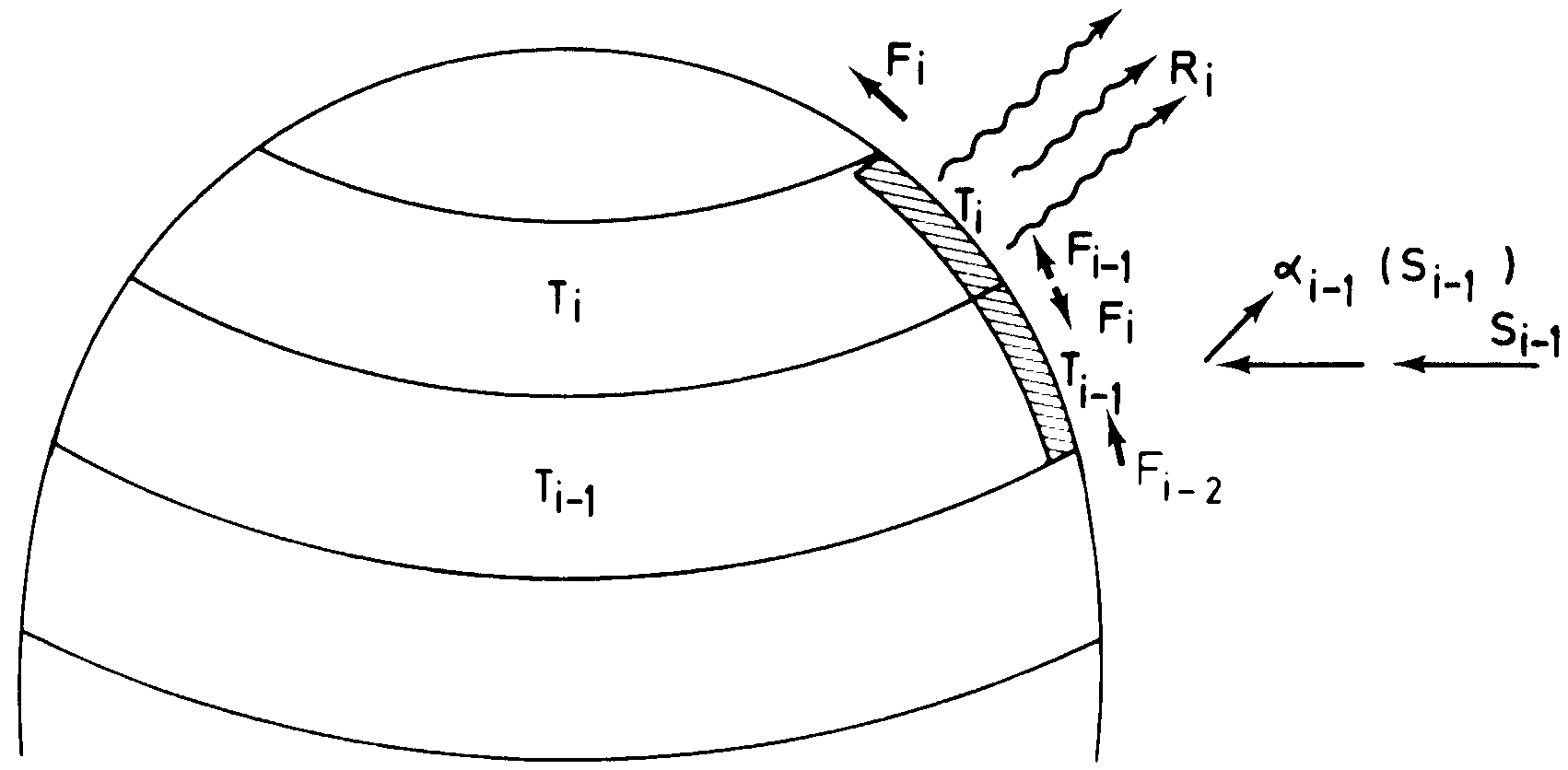
Instead of treating Earth as a single lump, we break it into latitudinal bands—like slicing an orange into horizontal rings. This allows us to model how energy moves between different regions rather than just considering a global average.

In this particular version, we divide the Northern Hemisphere into nine bands, each spanning 10 degrees of latitude. By doing so, we can study how different parts of the planet gain and lose heat, as well as how they exchange energy with their neighbors.

Heat flows: what’s going in, what’s going out

In an energy balance model, the main goal is to account for all heat flows in and out of the system. In the model we are examining, both the solar flux and albedo vary with latitude. The solar flux is denoted by $S_{i}$ and the albedo is denoted by $α_{i}$ , where i ranges from 1 to 9 representing different latitude bands. The incoming heat flow for our system would be:

P_{g ain} = \frac{S _{i} ( 1 - α _{i} )}{4}

According to Stefan-Boltzmann law, the outgoing longwave radiation is:

R_{i} = σ T_{i}^{4} = A + B T_{i}

where A and B are experiment parameters.

Furthermore, if a particular latitude band is colder or warmer than the average global temperature, there will be a heat flow into or out of that region. We make the assumption that this heat flow is linearly dependent on the temperature difference between the specific region and the global temperature. In other words, the heat flow can be represented as $k_{t}$ multiplied by the temperature difference $(T_{i} - T_{a vg})$ , where $k_{t}$ represents the diffusivity. The energy exchange among latitudinal bands is thus:

F_{i} = k_{t} (T_{i} - T a vg)

Energy balance gives us:

P_{g ain} = P_{l oss}

or:

S_{i} (1 - α (T_{i})) = R (T_{i}) + F (T_{i})

Therefore:

T_{i} = \frac{S _{i} ( 1 - α _{i} ) + k _{t} T _{a vg} - A}{B + k _{t}}

Some Python code…

Model parameters & Variables

no_latbands = 9                #number of latitude bands
EPSILON = 1.*10**-6   #Small value to check the stable condition of the Model

# infrared radiation
A = 204.                 #infrared cooling ($Wm^{-2}$)
B = 2.17                 #sigma*T^4 - a + bT, sigma: Stefan-Boltzmann constant
 
# heat transfer
K = 3.81                 #diffusivity ($Wm^{-2}$/degC) (for energy exchange among latitudinal bands)
 
# albedo parameterization
TEMP_C1 = 0.             #1st temperature threshold --> no ice cover (degC)
TEMP_C2 = -10.           #2nd temperature threshold --> complete ice cover (degC)
ALB_ICE_FREE = [0.23,0.24,0.25,0.29,0.35,0.40,0.46,0.50,0.50]
ALB_ICE = 0.62
 
# incoming solar radiation
S0 = 1368               #Solar constant ($Wm^{-2}$)
# SOL_FRAC = [0.30475,0.29725,0.28,0.25525,0.223,0.1925,0.156,0.13275,0.125]
SOL_FRAC = np.array([0.30475,0.29725,0.28,0.25525,0.223,0.1925,0.156,0.13275,0.125])
SOL_FLUX = S0*SOL_FRAC   #incoming solar flux at each latitudinal band
# SOL_FLUX = np.array(SOL_FLUX)

# Initiate zero arrays
no_latbands
# variables
alb = np.zeros(no_latbands)
temp = np.zeros(no_latbands)
temp_ini = np.zeros(no_latbands)
temp_pre = np.zeros(no_latbands)

Estimating surface area of each band

band_width = 90/no_latbands                                            # number of degrees in each zone
 
# midpoint of each band
lats = []                                                              
for i in np.arange(2.,90 - band_width/2.,band_width):
    lat = i
    lats.append(lat)
lats = np.array(lats)
 
# midpoint of each band in radians:
lats_rad = lats*np.pi/180
 
# half the number of radians in each band:
delta_rad = (np.pi/2)/no_latbands/2                          # =====> dp/2
 
# fraction of the surface of the sphere in each latitudinal band
lats_frac = np.sin(lats_rad + delta_rad) - np.sin(lats_rad - delta_rad)

Albedo for each band and mean albedo

The array alb is initially assigned the values of ALB_ICE_FREE, representing the albedo for each latitudinal band without ice cover. alb_sum is calculated by summing the product of each albedo value and its corresponding surface area fraction. alb_mean is obtained by dividing alb_sum by the sum of the surface area fractions.

alb = ALB_ICE_FREE
alb_sum = 0
for i in range(1,no_latbands+1):
    alb_sum += alb[i-1]*lats_frac[i-1]
alb_mean = alb_sum/sum(lats_frac)

Function for finding temperature

The code below defines a function called ebm1d (one-dimensional energy balance model) to find the equilibrium temperature for a planet with multiple latitudinal bands.

The function takes four input parameters: a, b, k, and i.
a, b, and k represent the parameters A, B, and K used in the energy balance equations.
i is a flag indicating whether the planet has ice cover (i = 1) or not (i = 0).

def ebm1d(a,b,k,i):
    global A, B, K, no_latbands, lats, alb, temp
 
    # set up iterations:
    temp[:] = ((S0/4.)*(1-alb_mean)-A)/B
    step_num = 1
    max_temp_diff = 1.
    tol_temp_diff = 1e-6
    max_steps=100
    
    A = a
    B = b
    K = k
 
    while (step_num<max_steps) and (max_temp_diff>tol_temp_diff):
        temp_pre = temp
        step_num+=1
 
        #calculate albedo:
        if i==1:
            alb[:] = ALB_ICE
            strg = 'icy'
        else:
            strg = 'not icy'
            for j in range(1,no_latbands+1):
                if (temp_pre[j-1] <= TEMP_C2):
                    alb[j-1] = ALB_ICE
                    # print('1')
                elif (temp_pre[j-1] > TEMP_C1):
                    alb[j-1] = ALB_ICE_FREE[j-1]
                    # print('2')
                else:
                    alb[j-1] = ALB_ICE + (ALB_ICE_FREE[j-1] - ALB_ICE)*(temp_pre[j-1] - TEMP_C2)/(TEMP_C2 - TEMP_C1)
                    # alb[j-1] = (TEMP_C1 - temp_pre[j-1])/(TEMP_C1 - TEMP_C2) * ALB_ICE + (temp_pre[j-1] - TEMP_C2)/(TEMP_C1 - TEMP_C2)*ALB_ICE_FREE[j-1]
                    # print('3')
        alb = np.array(alb)
        #update temperature:
        temp_avg = sum(np.multiply(lats_frac,temp))
        # print(alb)
        temp = (np.multiply(SOL_FLUX,(1-alb)) + K*temp_avg - A)/(B+K)
        max_temp_diff = max(abs(temp_pre - temp))
    array = np.array([lats,temp,alb])
    array = np.transpose(array)
    index_vals = np.arange(1,no_latbands+1,1)
    column_vals = ['Latitude (degree)','Equilibrium Temperature (degC)','Equilibrium Albedo']
    df = pd.DataFrame(data = array, index = index_vals, columns = column_vals)
    display(df)
    fig = plt.figure(figsize=(10,6))
    plt.plot(lats,temp,c='maroon',lw=2,label='Equil. Temperature (degC)')
 
    plt.title(f'Model A={A}, B={B}, K={K}, {strg}')
    plt.xticks(np.arange(0,95,5))
    # plt.yticks(np.arange())
    plt.legend()
    plt.grid()
    plt.show()

With the function created above, all we have to do now is to enter the parameters A, B, K and decide whether we want to find solar flux for the case Earth is entirely covered by ice or not.

Examples

Estimate the value of solar flux so that the Earth will be entirely covered by ice

For this case, I entered the values for A, B and K, and i = 1 to notify that this is an icy case. The solar flux for each latitudinal band can be found in the following table:

ebm1d(204.,2.17,3.81,1)

Latitude (degree)	Equil. Temperature (degC)	Equil. Albedo	Solar Flux
2.0	-33.298668	0.62	158.42124
12.0	-33.950642	0.62	154.52244
22.0	-35.450180	0.62	145.55520
32.0	-37.601692	0.62	132.68916
42.0	-40.405177	0.62	115.92432
52.0	-43.056535	0.62	100.06920
62.0	-46.229471	0.62	81.09504
72.0	-48.250588	0.62	69.00876
82.0	-48.924294	0.62	64.98000

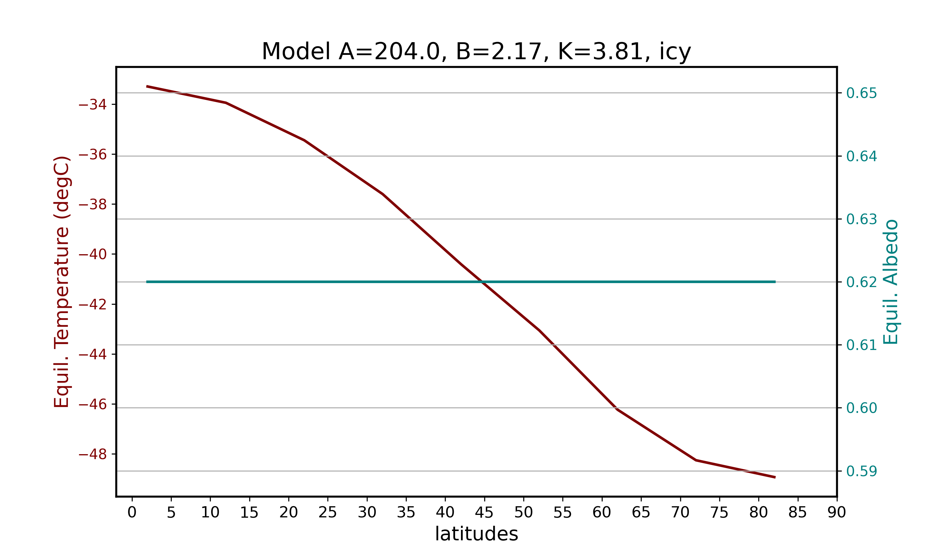Apparently, the equilibrium albedo remains constant at 0.62 for all bands because this is what I defined in the function for an icy planet (although I think this could be improved by defining more complex assumptions). The equilibrium temperatures and solar fluxes, on the other hand, both decreases with the increase in latitudes. We can also see that the temperatures are all extremely low (the highest temperature at the lowest latitude is only -33.3 $°$ C). This seems to be correct for the case of an icy planet.

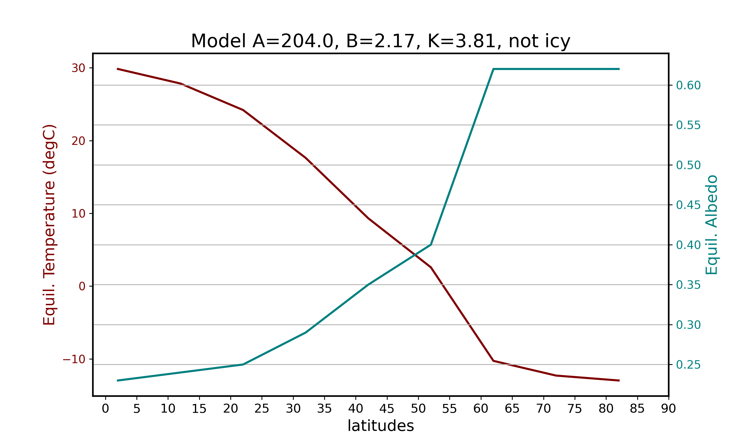
Different K values

Budyko (1969) let $k_{t} = 3.81$ .

ebm1d(204.,2.17,3.81,0)

Latitude (degree)	Equilibrium Temperature (degC)	Equilibrium Albedo	Solar Flux
2.0	29.843628	0.23	321.01146
12.0	27.842528	0.24	309.04488
22.0	24.202916	0.25	287.28000
32.0	17.620846	0.29	247.91922
42.0	9.321913	0.35	198.29160
52.0	2.584856	0.40	158.00400
62.0	-10.276174	0.62	81.09504
72.0	-12.297291	0.62	69.00876
82.0	-12.970997	0.62	64.98000

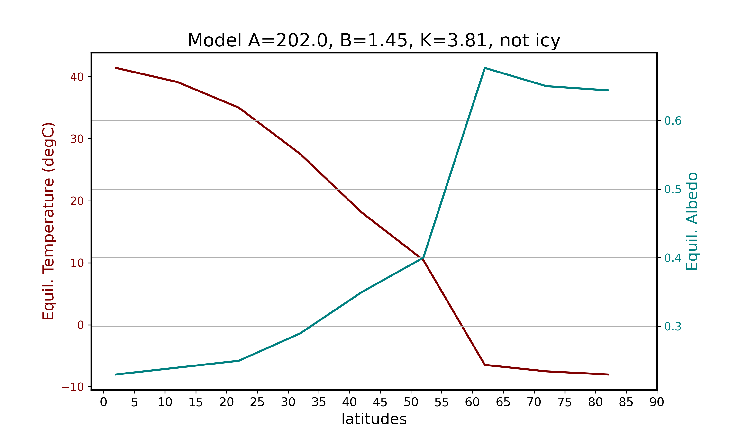
Different A and B values

Bydyko (1969) let $A = 202 W m^{- 2}$ and $B = 1.45 W m^{- 2} ° C^{- 1}$ .

ebm1d(202.,1.45,3.81,0)

Latitude (degree)	Equilibrium Temperature (degC)	Equilibrium Albedo	Solar Flux
2.0	41.426145	0.230000	321.011460
12.0	39.151130	0.240000	309.044880
22.0	35.013320	0.250000	287.280000
32.0	27.530282	0.290000	247.919220
42.0	18.095374	0.350000	198.291600
52.0	10.436134	0.400000	158.004000
62.0	-6.474147	0.676414	69.055919
72.0	-7.513339	0.649840	63.589770
82.0	-8.021052	0.643747	60.919200

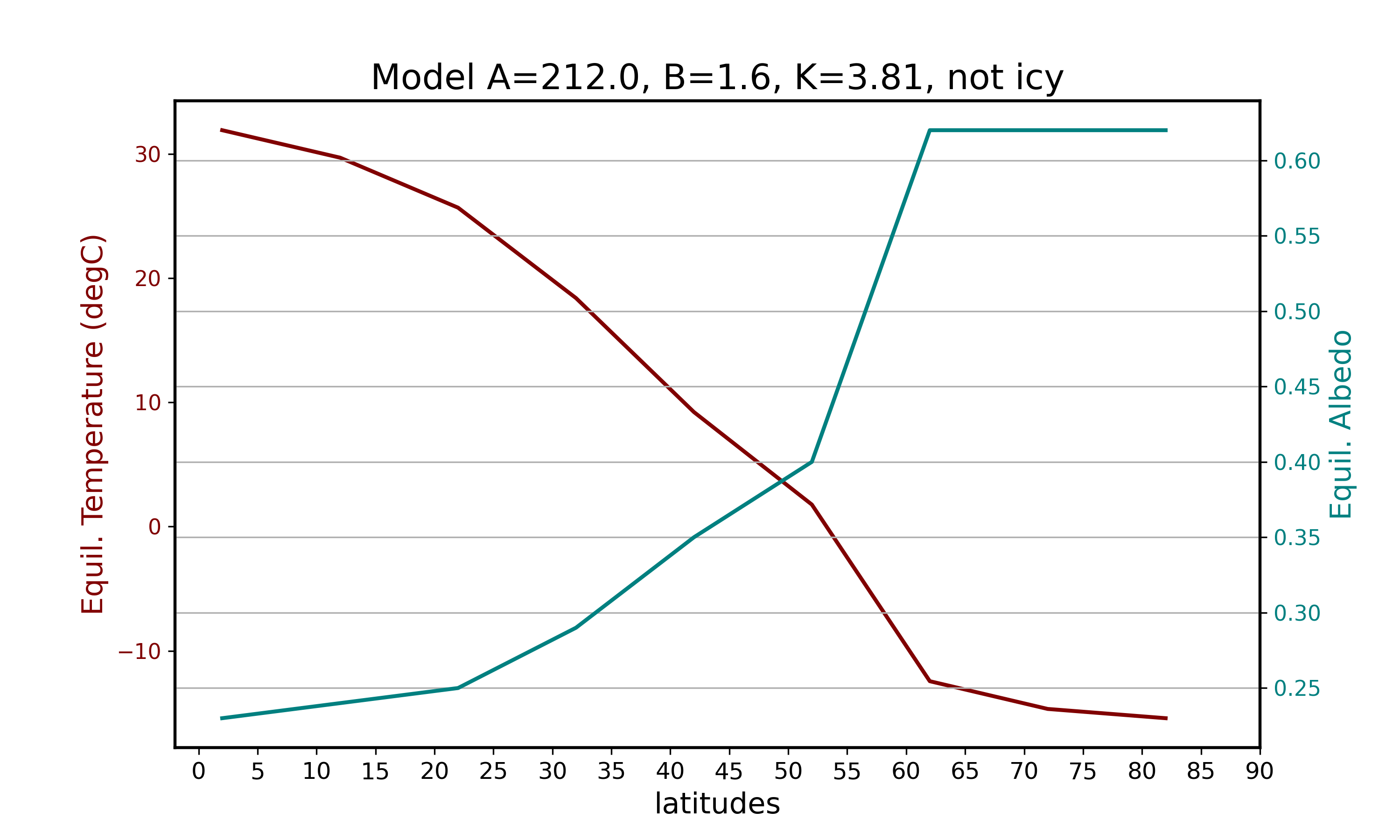
Cess (1976) let $A = 212 W m^{- 2}$ and $B = 1.6 W m^{- 2} ° C^{- 1}$ .

ebm1d(212.,1.6,3.81,0)

Latitude (degree)	Equilibrium Temperature (degC)	Equilibrium Albedo	Solar Flux
2.0	31.903027	0.23	321.01146
12.0	29.691090	0.24	309.04488
22.0	25.668006	0.25	287.28000
32.0	18.392446	0.29	247.91922
42.0	9.219134	0.35	198.29160
52.0	1.772258	0.40	158.00400
62.0	-12.443816	0.62	81.09504
72.0	-14.677879	0.62	69.00876
82.0	-15.422567	0.62	64.98000

L'arboretum

Explorer

Table of Contents

One-dimensional Energy Balance Model

The One-Dimensional Energy Balance Model

Heat flows: what’s going in, what’s going out

Some Python code…

Model parameters & Variables

Estimating surface area of each band

Function for finding temperature

Examples

Estimate the value of solar flux so that the Earth will be entirely covered by ice

Different K values

Different A and B values

💬 Logbook

🧭 Interactive Map

Backlinks

L'arboretum

Explorer

Table of Contents

One-dimensional Energy Balance Model

The One-Dimensional Energy Balance Model

Heat flows: what’s going in, what’s going out

Some Python code…

Model parameters & Variables

Estimating surface area of each band

Function for finding temperature

Examples

Estimate the value of solar flux so that the Earth will be entirely covered by ice

Different K values

Different A and B values

💬 Logbook

🧭 Interactive Map

Backlinks

🏷️ Tags