The Planet that regulates itself: Daisy World

Earth is kind of like one giant, living organism. At least, that’s what the Gaia Hypothesis suggests—it views the planet as a self-regulating system where the atmosphere, oceans, land, and life all work together to maintain conditions that sustain life itself. Everything is interconnected, and living organisms don’t just adapt to their environment—they actively shape it in ways that keep the system stable.

To explore this idea, James Lovelock and Andrew Watson introduced Daisyworld in 1983. It’s a super simplified, fictional planet designed to demonstrate how biological feedback can help regulate climate. Instead of dealing with complicated atmospheric chemistry or plate tectonics, Daisyworld just has… daisies. Two types, to be exact:

• Black daisies: These little guys have a low albedo (aka reflectivity), meaning they absorb more sunlight and warm up their surroundings.
• White daisies: These are the opposite—they have a high albedo and reflect sunlight, helping to cool things down.

The never-ending Daisy Dance

So, here’s how Daisyworld plays out:

1. In the beginning, the planet is cold, so black daisies thrive. They absorb heat, warming up the planet.
2. As temperatures rise, it gets too hot for black daisies. But now, it’s perfect for white daisies! So they take over.
3. More white daisies = more sunlight reflected back into space = cooling effect.
4. Eventually, it gets too cold for white daisies, but now black daisies can make a comeback… and the cycle repeats.

This back-and-forth keeps the planet’s temperature within a narrow, life-friendly range. It’s a beautiful example of a negative feedback loop, where initial changes get muted by the system itself, helping to maintain stability.

Earth’s own feedback loops

Obviously, Earth is way more complicated than Daisyworld. There’s rotation, seasons, geography, diseases, humans—the whole chaotic mix. But the same feedback principles apply.

For example, consider clouds. When temperatures rise, more water evaporates, forming clouds. And since clouds, like white daisies, have a high albedo, they reflect sunlight and help cool the planet—a natural negative feedback loop.

But not all feedback loops are stabilizing. Take polar ice and snow. They reflect a ton of sunlight, keeping the poles cool. But when global temperatures rise, ice melts, revealing darker ocean or land underneath—which absorbs more heat, melting even more ice. This is a positive feedback loop, where warming triggers more warming. And with climate change accelerating, the natural reflectivity of our icy poles is disappearing fast.

Daisyworld may be an imaginary planet, but it highlights something crucial: maintaining life on Earth depends on a delicate balance. Too much change—whether from natural cycles or human activities—can disrupt the system in ways that are hard to predict. If we want to keep our real-world Daisyworld livable, we have to understand and respect the feedback loops that keep our planet in check.

The model

Growth rate versus Temperature

Let’s have a look at the little code I made during a class on Climate Modelling:

Some parameters used in the code:

• S0: Solar constant (total solar irradiance received at the planet’s distance from the Sun).
• eps: Emissivity of the planet’s surface.
• sig: Stefan-Boltzmann constant.
• alb_w: Albedo of white daisies.
• alb_b: Albedo of black daisies.
• alb_g: Albedo of the available ground (unoccupied land).
• q: A constant used to calculate the local temperature based on the albedo.
• k: A constant determining the growth rate of daisies based on the temperature difference from T0.
• T0: The optimal temperature at which daisies grow most effectively.
• d: Death rate of daisies.

I created an array T that starts from 0 and increments by 0.1 until reaching 46. This array represents the range of temperatures over which the growth rates of daisies will be calculated.

The for loop iterates over each temperature value in T and calculates the growth rate of black and white daisies using a quadratic function (1 - k * (T0 - Tt) ** 2). The max(0, ...) function ensures that the growth rate does not go below zero. The calculated growth rates are stored in the fb_list and fw_list lists.

S0 = 1000
eps = 0.3
sig = 5.67*10**(-8)
alb_w = 0.75
alb_b = 0.25
alb_g = 0.5
q = 20
k = 0.003265
T0 = 22.5
d = 0.3
 
tolerance = 1.*10**(-6)
diff = 1.0

b_list = []
w_list = []
 
x_list = []
alb_p_list = []
Te_list = []
Tb_list = []
Tw_list = []
fb_list = []
fw_list = []
db_list = []
dw_list = []
 
T = np.arange(0,46,0.1)
for Tt in T:
    fb = max(0,1 - k*(T0 - Tt)**2)
    fw = max(0,1 - k*(T0 - Tt)**2)
    
    fb_list.append(fb)
    fw_list.append(fw)
    
fig = plt.figure(figsize=(20,6))
 
ax = fig.add_subplot(1,2,1)
ax.plot(T, fb_list,'maroon',lw=3)
ax.set_title('Black daisy')
ax.set_xlabel('Temperature')
ax.set_ylabel('Growth rate')
ax.grid()
 
ax = fig.add_subplot(1,2,2)
ax.plot(T, fb_list,'goldenrod',lw=3)
ax.set_title('White daisy')
ax.set_xlabel('Temperature')
ax.grid()
 
plt.savefig('06_growthrate.png',dpi=300)
plt.show()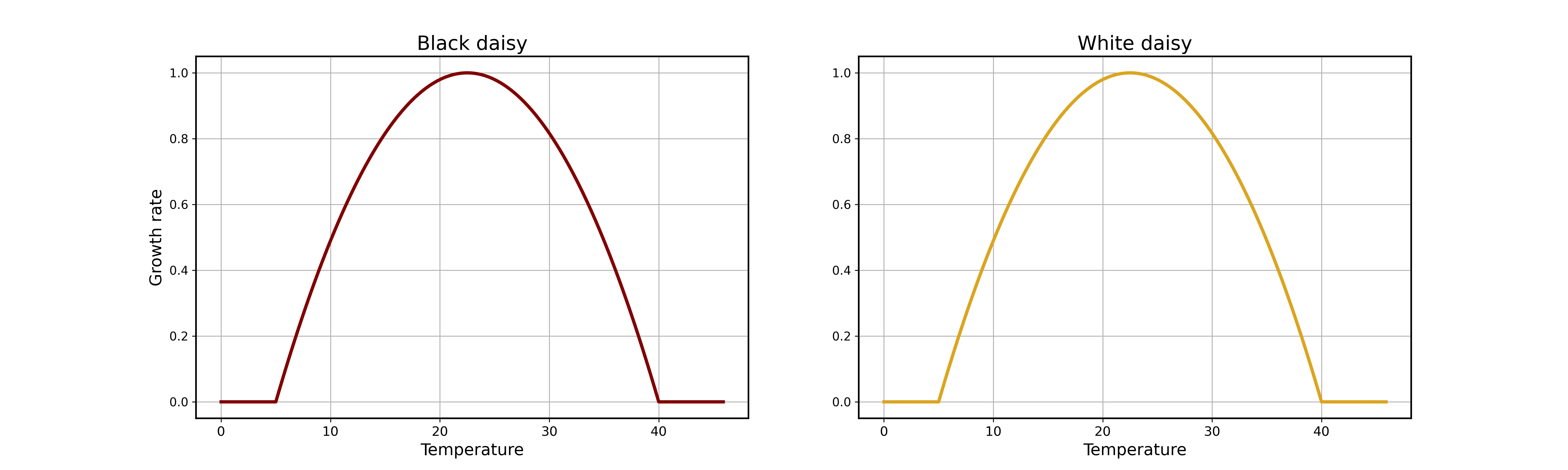

Obviously, the growth rate plots of both types of daisies follow the same pattern.

Equilibrium b and w values at S = S0 = 1000, with initial b = w = 0.2

Next, I calculated the equilibrium values for the variables b and w in the model when the solar constant S is equal to S0 = 1000, with initial values of b and w set to 0.2.

The while loop:

• diff and tolerance are variables used to determine when to stop the loop. The loop continues as long as the absolute value of the sum of dw and db is greater than tolerance.
• x = 1 - b - w: Calculates the proportion of unoccupied land (x) by subtracting the sum of b and w from 1.
• alb_p = w * alb_w + b * alb_b + x * alb_g: Calculates the planetary albedo (alb_p) by multiplying the albedo of white daisies (alb_w), black daisies (alb_b), and the available ground (alb_g) by their respective proportions and summing them up.
• Te = (((1 - alb_p) * S0) / (4 * eps * sig)) ** (1. / 4) - 273.15: Computes the equilibrium temperature (Te) of the planet by using the Stefan-Boltzmann law. The result is then converted from Kelvin to Celsius by subtracting 273.15.
• Tb = Te + q * (alb_p - alb_b): Calculates the temperature of black daisies (Tb) by adding the equilibrium temperature (Te) to the product of q (a constant) and the difference between the planetary albedo (alb_p) and the albedo of black daisies (alb_b).
• Tw = Te + q * (alb_p - alb_w): Computes the temperature of white daisies (Tw) using the same formula as for Tb, but using the albedo of white daisies (alb_w) instead.
• fb = max(0, 1 - k * (T0 - Tb) ** 2): Calculates the growth rate of black daisies (fb) using a quadratic function (1 - k * (T0 - Tb) ** 2). It ensures that the growth rate does not go below zero.
• fw = max(0, 1 - k * (T0 - Tw) ** 2): Computes the growth rate of white daisies (fw) using the same quadratic function as for fb, but using the temperature of white daisies (Tw) instead.
• db = b * (x * fb - d): Calculates the change in the black daisy population (db) by multiplying the proportion of black daisies (b) by the difference between the product of x and fb and the death rate (d).
• dw = w * (x * fw - d): Computes the change in the white daisy population (dw) using the same formula as for db, but with the proportion of white daisies (w) and the growth rate of white daisies (fw).
• b += db and w += dw: Updates the values of b and w by adding the respective changes calculated in the previous steps.
• diff = abs(dw + db): Calculates the absolute difference between dw and db and assigns it to diff. This difference is used to determine whether the loop should continue or stop.

b = w = 0.2
while (diff>tolerance):
    x = 1 - b - w
    alb_p = w*alb_w + b*alb_b + x*alb_g
    Te = (((1-alb_p)*S0)/(4*eps*sig))**(1./4) - 273.15
    Tb = Te + q*(alb_p - alb_b)
    Tw = Te + q*(alb_p - alb_w)
    fb = max(0,1-k*(T0 - Tb)**2)
    fw = max(0,1-k*(T0 - Tw)**2)
    db = b*(x*fb - d)
    dw = w*(x*fw - d)
    b+=db
    w+=dw
 
    diff = abs(dw+db)
 
print('Equilibrium b and w is: ',b,w)

Equilibrium b and w is:  0.3828564993464297 0.2904829937848562

Based on these results, we can infer that in this specific Daisyworld model, the equilibrium state corresponds to a higher proportion of black daisies (b) compared to white daisies (w).

Daisyworld with varying S/S0

The code below is an extension of the previous Daisyworld model. It calculates the equilibrium values of various variables, such as the areas of black and white daisies (b_list and w_list), the uncovered area (x_list), the planetary temperatures with and without daisies (Te_list and Te_no_list), for different solar flux ratios (S/S0).

I defined a function daisy(sflux) that calculates the equilibrium values for a given solar flux ratio (sflux). It contains the same logic as the previous code but with slight modifications. Next, I determined the range and step size for the solar flux ratio loop.

The first for loop calculates the equilibrium values for the solar flux ratios ranging from 1.0 to ratio_min (0.39) in reverse order. It initializes b and w to 0.2 and calls the daisy() function with the current solar flux ratio (sr). The value of j is set to 1, indicating that the appended values will be in reverse order.

Similarly, the second for loop calculates the equilibrium values for the solar flux ratios ranging from 1.01 to ratio_max (1.6) in regular order. It initializes b and w to 0.2 and calls the daisy() function with the current solar flux ratio (sr). The value of j is set to 0, indicating that the appended values will be in regular order.

b_list = []
w_list = []
 
x_list = []
alb_p_list = []
Te_list = []
Tb_list = []
Tw_list = []
fb_list = []
fw_list = []
db_list = []
dw_list = []
Te_no_list = []
 
def daisy(sflux):
    global b,w,j, b_list, w_list, x_list, Tb_list, Tw_list, Te_list, Te_no_list
    
    diff = 1.0
    S = S0*sflux
 
    while (diff>tolerance):
        x = 1 - b - w
        alb_p = w*alb_w + b*alb_b + x*alb_g
        Te = ((1-alb_p)*S/(sig))**(1./4) - 273.15
        Tb = Te + q*(alb_p - alb_b)
        Tw = Te + q*(alb_p - alb_w)
        fb = max(0,1-k*(T0 - Tb)**2)
        fw = max(0,1-k*(T0 - Tw)**2)
        db = b*(x*fb - d)
        dw = w*(x*fw - d)
        b+=db
        w+=dw
        
        diff = abs(dw)+abs(db)
    Te_no = ((1-alb_g)*S/(sig))**(1./4) - 273.15
 
    if j == 0:
        b_list.append(b)
        w_list.append(w)
        x_list.append(x)
        Tb_list.append(Tb)
        Tw_list.append(Tw)
        Te_list.append(Te)
        Te_no_list.append(Te_no)
    else:
        b_list.insert(0,b)
        w_list.insert(0,w)
        x_list.insert(0,x)
        Tb_list.insert(0,Tb)
        Tw_list.insert(0,Tw)
        Te_list.insert(0,Te)
        Te_no_list.insert(0,Te_no)
        
 
ratio_max = 1.6
ratio_min = 0.39
ratio_step = 0.01
 
""" S/S0 ratio loop is cut into 2 loops (at S/S0 = 1.0):
From 0.4 to 1.0, the variables are updated backwards: from larger S/S0 value to smaller value
          For solar fluxes smaller than initial solar flux value, the model is a cooling process
From 1.01 to 1.6, the variables are updated forwards: from smaller S/S0 value to larger value
          For solar fluxes larger than initial solar flux value, the model is a warming process"""
 
b=w=0.2                                         # initialize b = w = 0.1
for sr in np.arange(1.,ratio_min,-ratio_step):  # for S/S0 from 1.0 -> 0.4:
    j=1                                         # diff = 1 at beginning of every for loop, while (x -> alb_p -> Te -> ... -> b and w -> diff changing); append backward
    daisy(sr)
 
b=w=0.2                                         # initialize b = w = 0.1
for sr in np.arange(1.01,ratio_max,ratio_step): # for S/S0 from 1.01 ->  1.6: 
    j=0                                         # diff = 1 at beginning of every for loop, while (x -> alb_p -> Te -> ... -> b and w -> diff changing); append
    daisy(sr)
   
sratios = np.arange(0.4,1.61,0.01)
fig = plt.figure(figsize=(20,6))
 
ax = fig.add_subplot(1,2,1)
ax.plot(sratios,b_list,color='maroon',lw=3,label='Black daisy area')
ax.plot(sratios,w_list,color='goldenrod',lw=3,label='White daisy area')
ax.plot(sratios,x_list,'k',lw=2,ls='--',label='Uncovered area')
ax.set_title('Equilibrium area of black/white daisy vs S/S0')
ax.set_xlabel('S/S0')
ax.set_ylabel('Area')
ax.set_xticks(np.arange(0.4,1.7,0.1))
ax.set_yticks(np.arange(0,1.1,0.1))
ax.legend()
ax.grid(True)
 
ax = fig.add_subplot(1,2,2)
ax.plot(sratios,Te_list,lw=3,color='goldenrod',label='Equil temperature (with daisy)')
ax.plot(sratios,Te_no_list,lw=2,color='k',ls='--',label='Equil temperature (without daisy)')
ax.set_title('Planetary temperature (with and without daisy) vs S/S0')
ax.set_xlabel('S/S0')
ax.set_ylabel('Temperature')
ax.set_xticks(np.arange(0.4,1.7,0.1))
ax.set_yticks(np.arange(-30,80,10))
ax.legend()
ax.grid(True)
 
plt.savefig('06_equi-area-temp_vs_Sratio.png',dpi=300)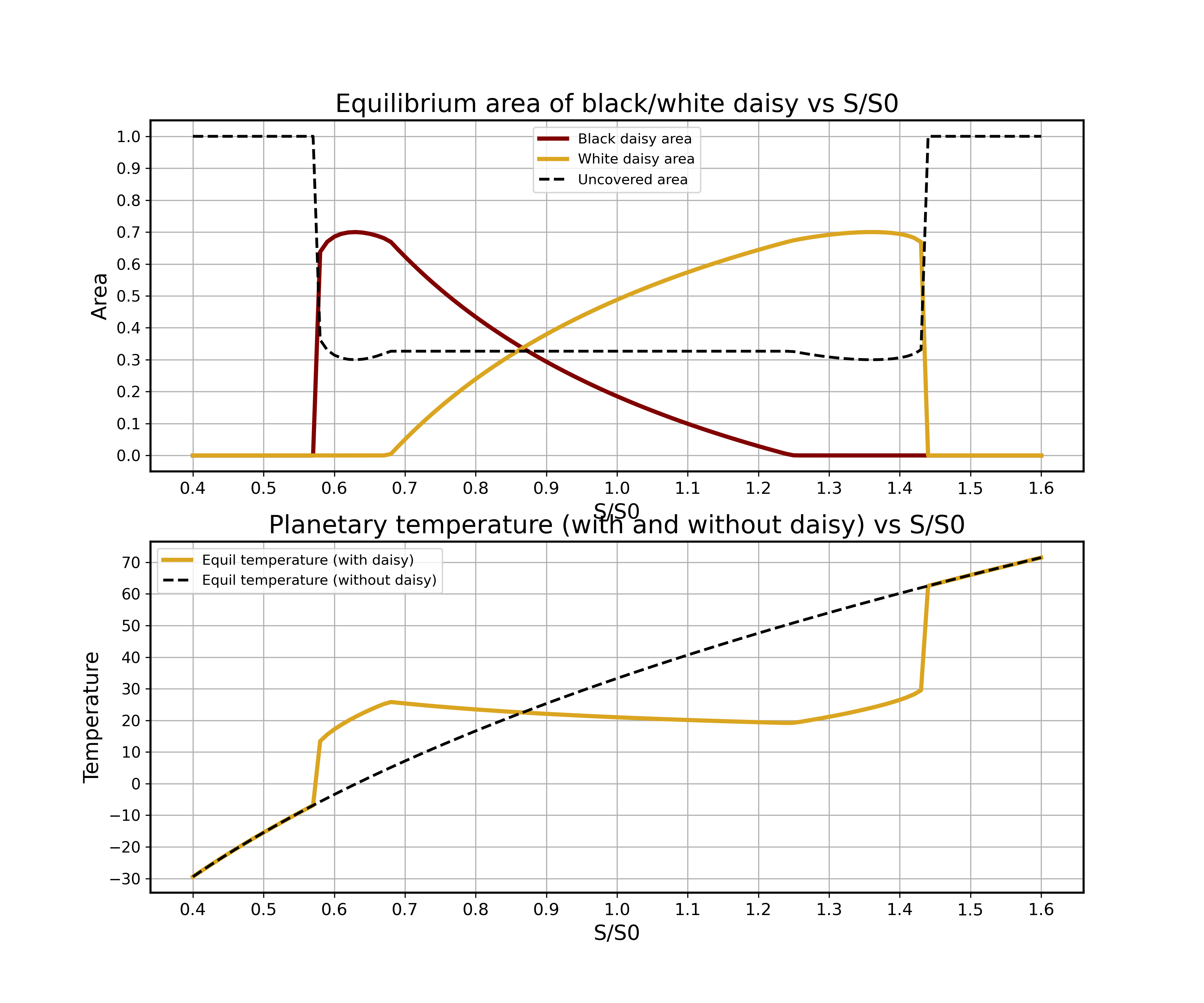

The use of two for loops in the code is due to the specific design of the Daisyworld model and the way it handles different solar flux ratios. The first for loop represents the cooling phase of the model. By decreasing the solar flux ratio, the model simulates a cooling process where the solar energy reaching the planet is gradually reduced. The second for loop represents the warming phase of the model. By increasing the solar flux ratio, the model simulates a warming process where the solar energy reaching the planet is gradually increased.

Daisyworld with only black daisies

The code below is a modified version of the Daisyworld model that considers only black daisies.

b_list = []
x_list = []
alb_p_list = []
Te_list = []
Tb_list = []
fb_list = []
db_list = []
Te_no_list = []
 
def daisy(sflux):
    global b,w,j, b_list, w_list, x_list, Tb_list, Tw_list, Te_list, Te_no_list
    
    diff = 1.0
    S = S0*sflux
 
    while (diff>tolerance):
        x = 1 - b
        alb_p = b*alb_b + x*alb_g
        Te = ((1-alb_p)*S/(sig))**(1./4) - 273.15
        Tb = Te + q*(alb_p - alb_b)
        fb = max(0,1-k*(T0 - Tb)**2)
        db = b*(x*fb - d)
        b+=db
        
        diff = abs(db)
    Te_no = ((1-alb_g)*S/(sig))**(1./4) - 273.15
 
    if j == 0:
        b_list.append(b)
        x_list.append(x)
        Tb_list.append(Tb)
        Te_list.append(Te)
        Te_no_list.append(Te_no)
    else:
        b_list.insert(0,b)
        x_list.insert(0,x)
        Tb_list.insert(0,Tb)
        Te_list.insert(0,Te)
        Te_no_list.insert(0,Te_no)
        
 
ratio_max = 1.6
ratio_min = 0.39
ratio_step = 0.01
 
""" S/S0 ratio loop is cut into 2 loops (at S/S0 = 1.0):
From 0.4 to 1.0, the variables are updated backwards: from larger S/S0 value to smaller value
          For solar fluxes smaller than initial solar flux value, the model is a cooling process
From 1.01 to 1.6, the variables are updated forwards: from smaller S/S0 value to larger value
          For solar fluxes larger than initial solar flux value, the model is a warming process"""
 
b=w=0.2                                         # initialize b = w = 0.1
for sr in np.arange(1.,ratio_min,-ratio_step):  # for S/S0 from 1.0 -> 0.4:
    j=1                                         # diff = 1 at beginning of every for loop, while (x -> alb_p -> Te -> ... -> b and w -> diff changing); append backward
    daisy(sr)
 
b=w=0.2                                         # initialize b = w = 0.1
for sr in np.arange(1.01,ratio_max,ratio_step): # for S/S0 from 1.01 ->  1.6: 
    j=0                                         # diff = 1 at beginning of every for loop, while (x -> alb_p -> Te -> ... -> b and w -> diff changing); append
    daisy(sr)
   
sratios = np.arange(0.4,1.61,0.01)
fig = plt.figure(figsize=(20,6))
 
ax = fig.add_subplot(1,2,1)
ax.plot(sratios,b_list,color='maroon',lw=3,label='Black daisy area')
ax.plot(sratios,x_list,'k',lw=2,ls='--',label='Uncovered area')
ax.set_title('Equilibrium area of black daisy vs S/S0')
ax.set_xlabel('S/S0')
ax.set_ylabel('Area')
ax.set_xticks(np.arange(0.4,1.7,0.1))
ax.set_yticks(np.arange(0,1.1,0.1))
ax.legend()
ax.grid(True)
 
ax = fig.add_subplot(1,2,2)
ax.plot(sratios,Te_list,lw=3,color='goldenrod',label='Equil temperature (with daisy)')
ax.plot(sratios,Te_no_list,lw=2,color='k',ls='--',label='Equil temperature (without daisy)')
ax.set_title('Planetary temperature (with and without black daisy) vs S/S0')
ax.set_xlabel('S/S0')
ax.set_ylabel('Temperature')
ax.set_xticks(np.arange(0.4,1.7,0.1))
ax.set_yticks(np.arange(-30,80,10))
ax.legend()
ax.grid(True)
 
plt.savefig('06_blackonly.png',dpi=300)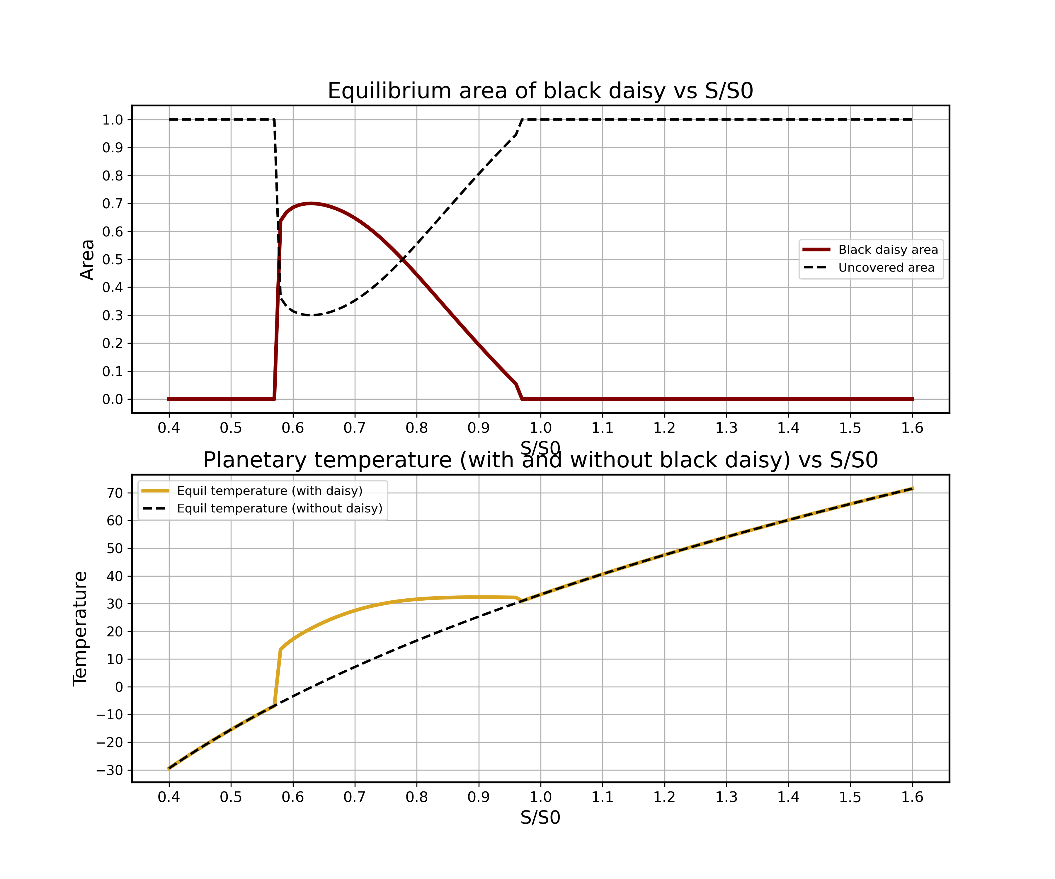

The equilibrium area of black daisies (b_list) would be the sole variable representing the daisy population. The absence of white daisies means that there is no competition or interaction between black and white daisies for resources or space. As a result, the equilibrium area of black daisies would solely depend on the solar flux ratio and other parameters specific to black daisies. The variable representing the uncovered area (x_list) would still be present, but its dynamics and equilibrium value would differ compared to the model with both black and white daisies. In this case, the uncovered area would represent the non-daisy-covered land, and its value would be inversely related to the area of black daisies.

With only black daisies present, the self-regulation of the planetary temperature would mainly depend on the albedo of the black daisies and the solar flux ratio. The population of black daisies would grow or decline based on the interplay between the growth rate function and death rate (d).