NDWI Segmentation Threshold in Image Processing

Image segmentation is frequently used in digital image processing and analysis to divide a digital image into a number of regions of pixels, usually based on the properties of the pixels in the image. For instance, picture segmentation might be used to distinguish between the foreground and background or to group together clusters of pixels that have a common color or shape.

Thresholding is a method that refers to a common approach of finding similarities between regions of an image. Here, we alter an image’s pixel characteristics to make it simpler to analyze. We turn a grayscale or RGB image into a binary image (only black and white, for example). Thresholding allows us to select the areas of an image that are of interest while disregarding the other parts. For instance, using a satellite image, this technique may be used to identify areas of surface water! Isn’t it interesting how we can separate and highlight water regions on a planet from satellite images? In this post, I’ll give a brief overview of the principles and how ENVI can be used to implement it. I never really dived deep into remote sensing subjects though so I could be wrong, do tell me!

Principles

There are a few important concepts for segmentation thresholding using NDWI/NDVI.

Digital Number (DN)

A digital image is a matrix made of pixels (picture elements). Each pixel is filled by an integer called a digital number. The digital number represents the radiance of the light measured for the pixel, and it is proportional to the radiance. A 256x256 spatial domain image, for example, has 256 x 256 = 65,536 pixels, whereas a 1024x1280 image has 1,310,720 pixels. The value of each pixel in grayscale images is related to the amount of bits of data used to represent the pixel (typically 8 bits), ranging from 0 to 255 (2⁸ = 256 grayscale levels created from combinations of 8 binary numbers: 00000000 to 11111111). If a pixel’s value is represented by 16 bits, the value range is 0 to 65,535 (2¹⁶ = 65,536 grayscale levels).

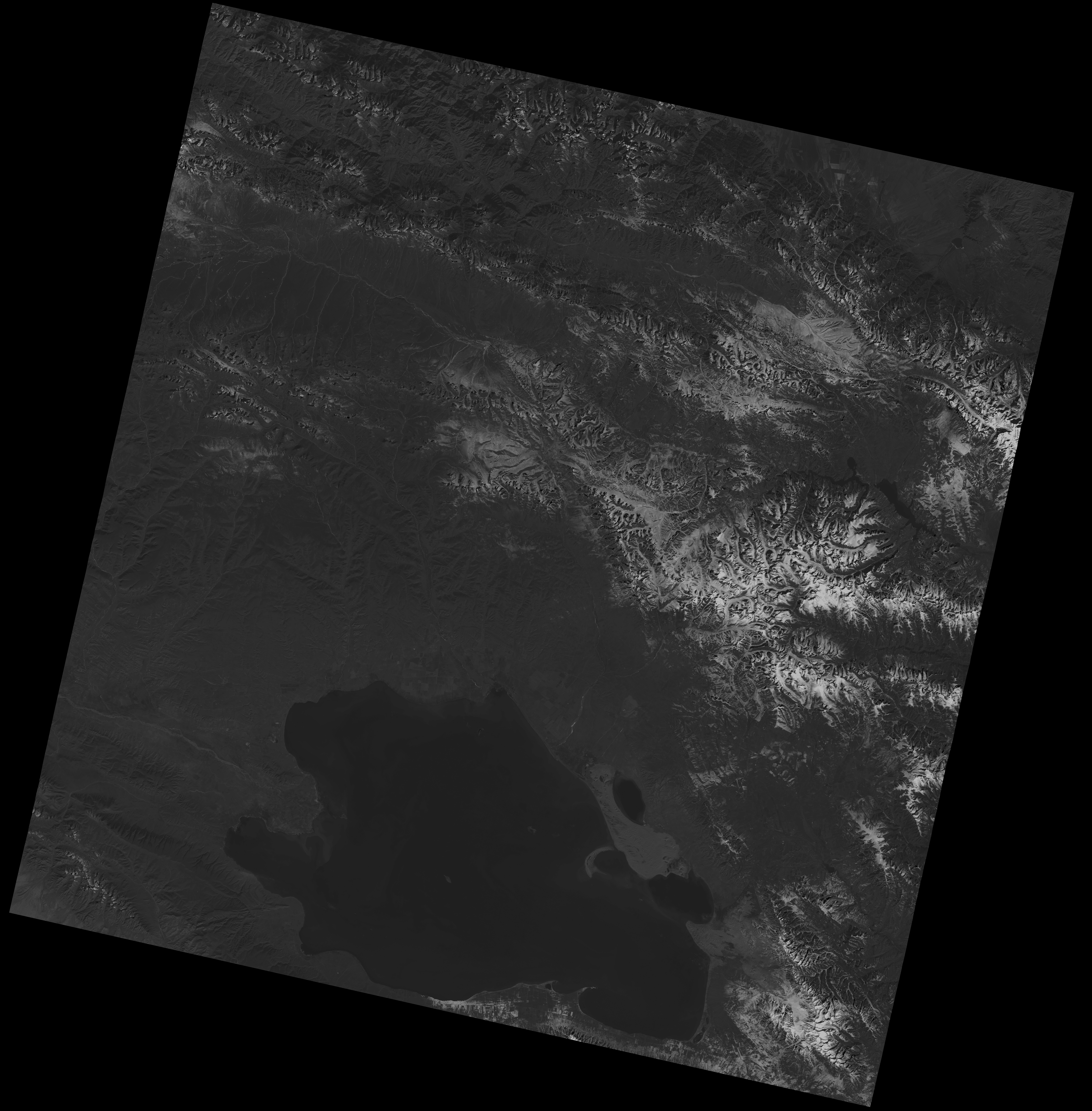
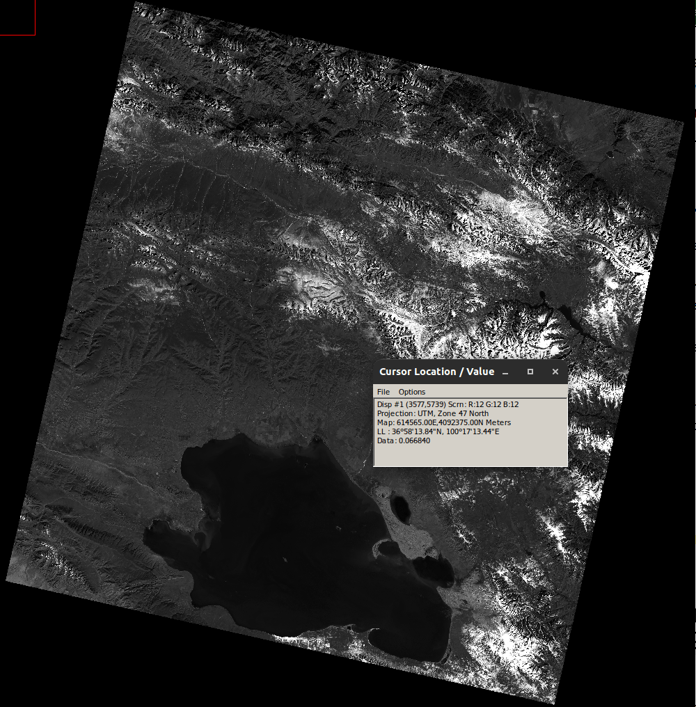
LANDSAT 8-9 image of Qinghai Lake (China) in the visible green band (Band 3)

You can have a look at the properties of this image using QGIS or many other applications.

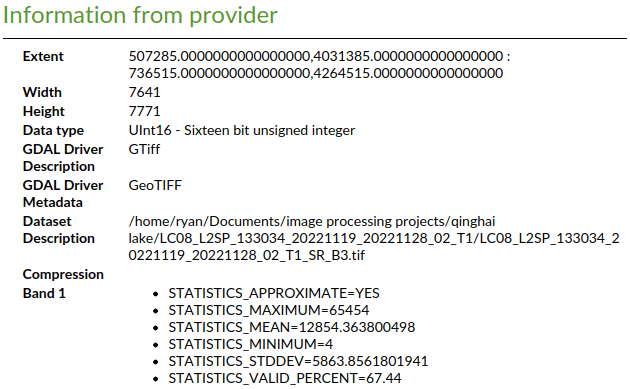
So this is a 16-bit image, which means the value range of each pixel would be from 0 to 65,535, representing the intensity of visible green light. For this particular image, the minimum value of a pixel is 4 (not completely “black”) and the maximum value is 65,454.

If you open this image in ENVI and access the cursor value, the number for data is the digital number of the pixel where your cursor is hovering.
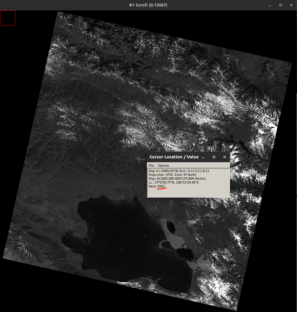
Here, my cursor is pointing at a pixel with a digital number of 8267

Digital numbers correspond to the energy detected and measured at the sensor. They are connected to surface reflectance values, but they are NOT the same! Using DNs collected by satellite without adjusting for atmospheric effects as light passes through the atmosphere may result in many problems!

Then what do we use instead?

Top of Atmosphere (TOA)

Remote sensing instruments directly measure radiance. This includes radiation reflected from the surface, as well as radiation reflected from nearby pixels, and perhaps most significantly, radiation reflected from clouds! Furthermore, radiance is affected not only by the intensity and direction of the target’s illumination, but also by its orientation and position.

Read more about the energy transfer in the atmosphere through my posts on climate and weather

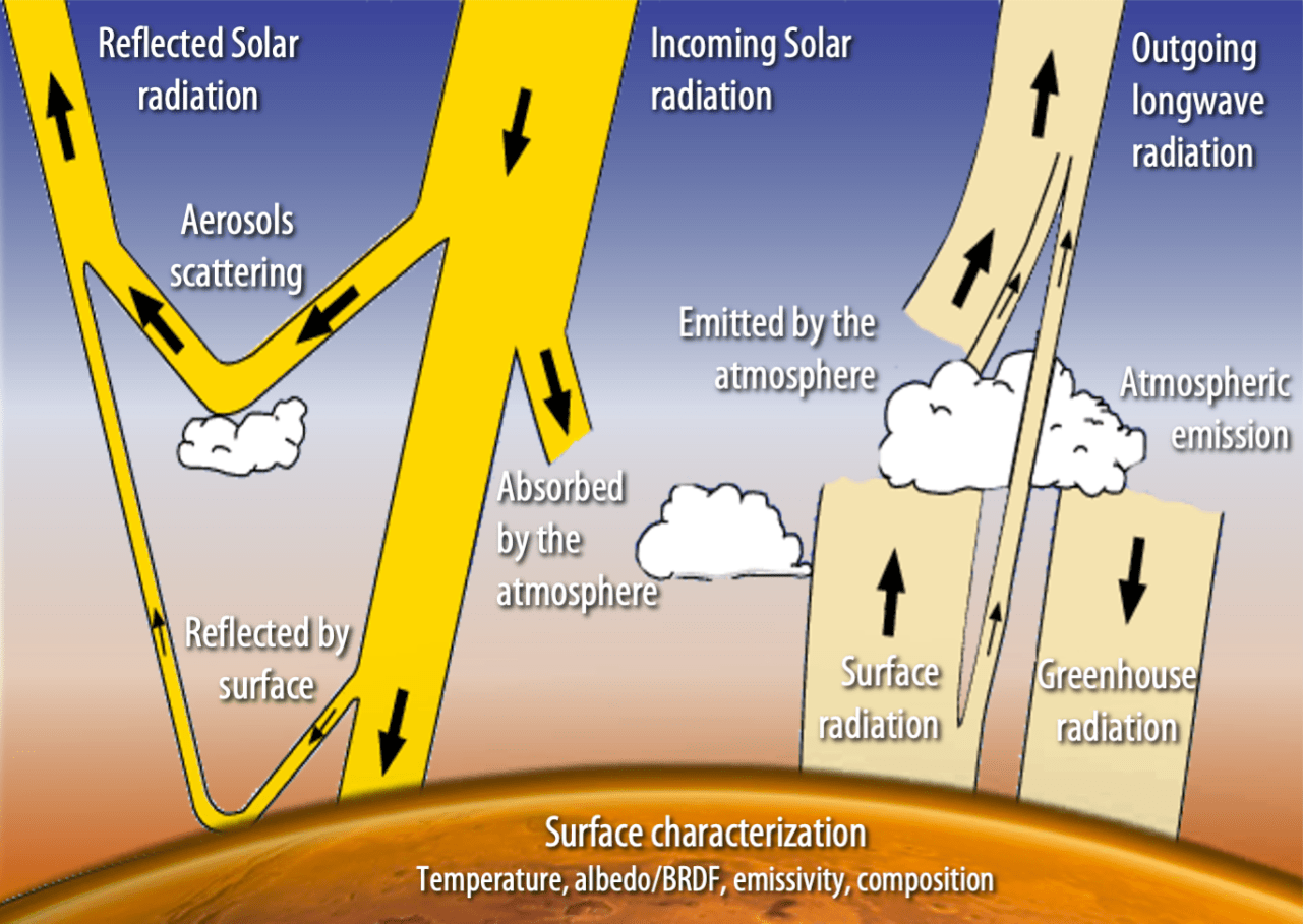
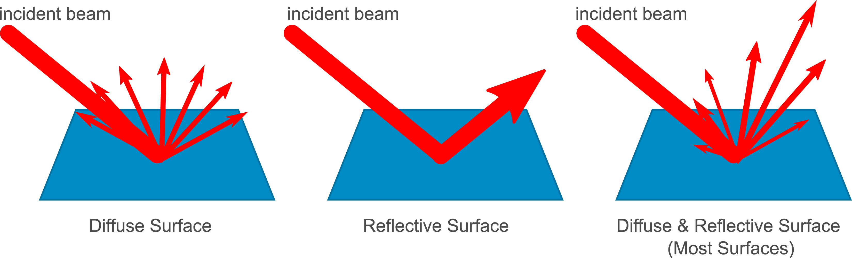
In other words, the travel of light in the atmosphere is influenced by a variety of elements as it goes down to the Earth through the atmosphere, diffusively reflects off the Earth’s surface, and then returns up through the atmosphere, suffering from scattering effects. Thus, instead of the digital number, we would determine the Top of Atmosphere (TOA) reflectance values, which can be estimated mainly from radiance leaving the ground, transmission factors and path radiance.

Reflectance values range from 0 to 1 and are stored in floating point data format. With ENVI, you can easily convert Landsat optical band data from the USGS in the “USGS GeoTIFF with Metadata” format to TOA reflectance values when you open the USGS file that ends with “MLT.TXT”. More details can be found in Section 1 of this page.

The metadata file “MLT.TXT” provides rescaling factors and parameters that can be used to manually convert Landsat data to TOA reflectance with the following formula, using the tool Band Math.

$${\rho }_{\lambda }=\frac{M_{\rho }{Q}_{cal}+A_{\rho }}{cos({\theta }_{SZ})}=\frac{M_{\rho }{Q}_{cal}+A_{\rho }}{sin({\theta }_{SE})}$$

where:

• $M_{\rho }$ is the band-specific multiplicative rescaling factor (REFLECTANCE_MULT_BAND_x in the metadata, where x is the band number).
• $A_{\rho }$ is the band-specific additive rescaling factor (REFLECTANCE_ADD_BAND_x).
• $Q_{cal}$ is the quantized and calibrated standard product pixel values (digital number DN).
• $M_{\rho }{Q}_{cal}+A_{\rho }$ is then the TOA planetary reflectance without correction for solar angle.
• ${\theta }_{SE}$ is the local sun elevation angle (SUN_ELEVATION)
• ${\theta }_{SZ}$ is the local solar zenith angle; ${\theta }_{SZ}=90°-{\theta }_{SE}$

And below is the result I got after converting from DN to TOA. You can see that the cursor value for data has changed. Its range (originally 0 to 65,535) is now from -1 to 1.

NDVI and NDWI

NDVI stands for Normalized Difference Vegetation Index and NDWI stands for Normalized Difference Water Index.

The Normalized Difference Vegetation Index (NDVI) is used to evaluate vegetation greenness and is important in evaluating vegetation density. The difference in near-infrared (which plant significantly reflects) and red light (which plant absorbs) is used to quantify vegetation.

$$NDVI=\frac{NIR-Red}{NIR+Red}$$

On the other hand, the Normalized Difference Water Index (NDWI) is used to evaluate changes in water content in bodies of water. Because water bodies absorb light substantially in the visible to infrared electromagnetic radiation spectrum, NDWI highlights water bodies using green and near-infrared wavelengths.

$$NDWI=\frac{Green-NIR}{Green+NIR}$$

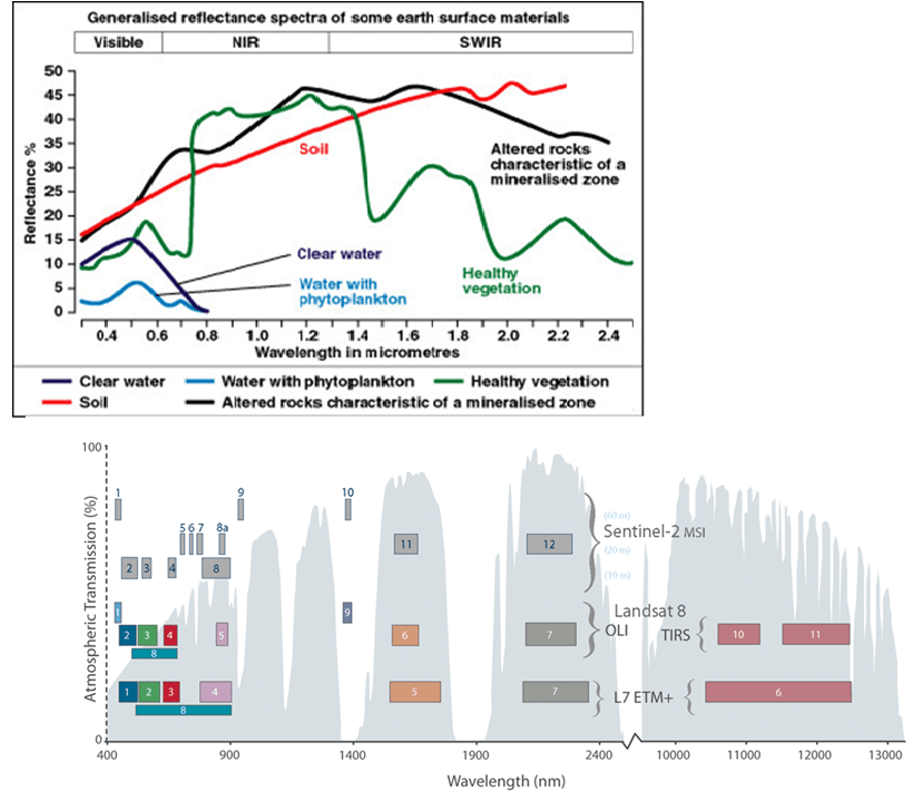
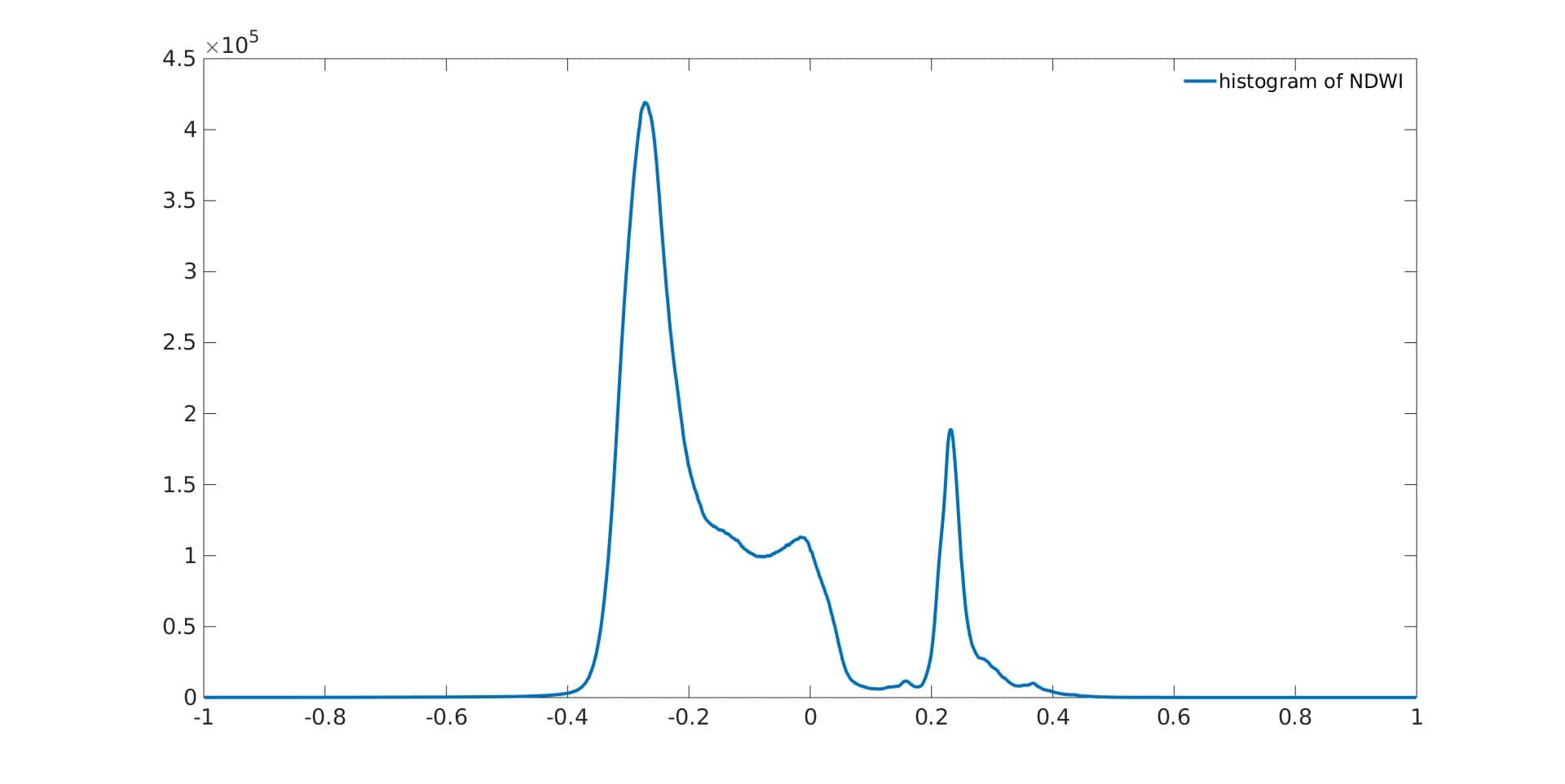
From the above figure, it is apparent that reflection in NIR wavelength over water bodies is lower than reflection in the Red wavelength. As a result, water bodies will have negative NDVI values. On the contrary, reflection in Green wavelength over water bodies is higher than reflection in NIR wavelength. Thus, water bodies will have positive NDWI values.

For Landsat 8, band 3 represents visible green light, band 4 represents visible red light and the near-infrared is shown in band 5. Therefore, for Landsat 8 data, we can calculate the NDVI and NDWI like below:

$$NDVI=\frac{B5-B4}{B5+B4}$$ $$NDWI=\frac{B3-B5}{B3+B5}$$

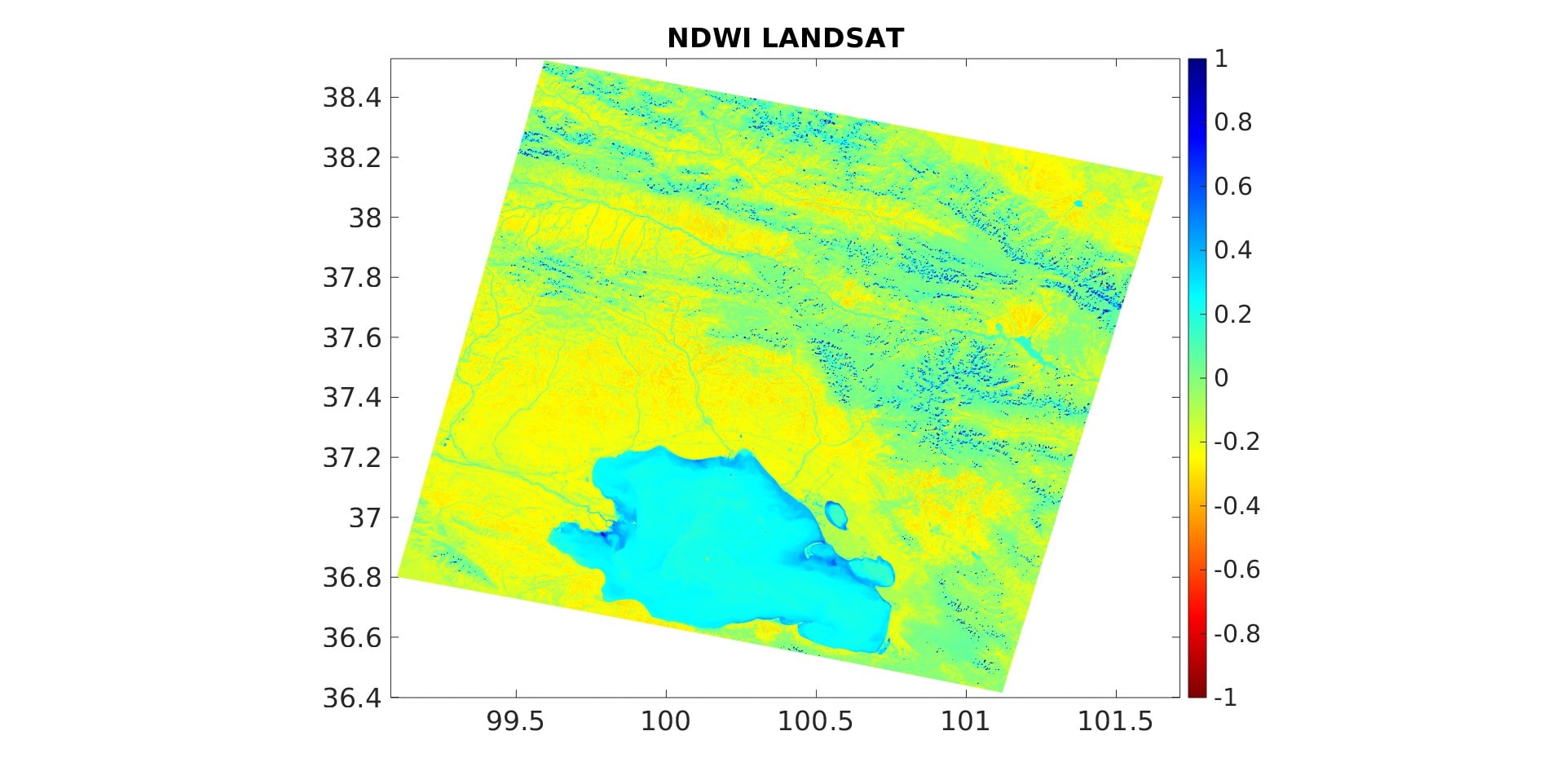
Using the NDVI tool on a layerstacked image (for example, layerstacking band 3 and band 5 to calculate NDWI), we can obtain the following result:

The cursor is hovering over Qinghai lake so we have positive NDWI value (I imported the NDWI file into the blue band)

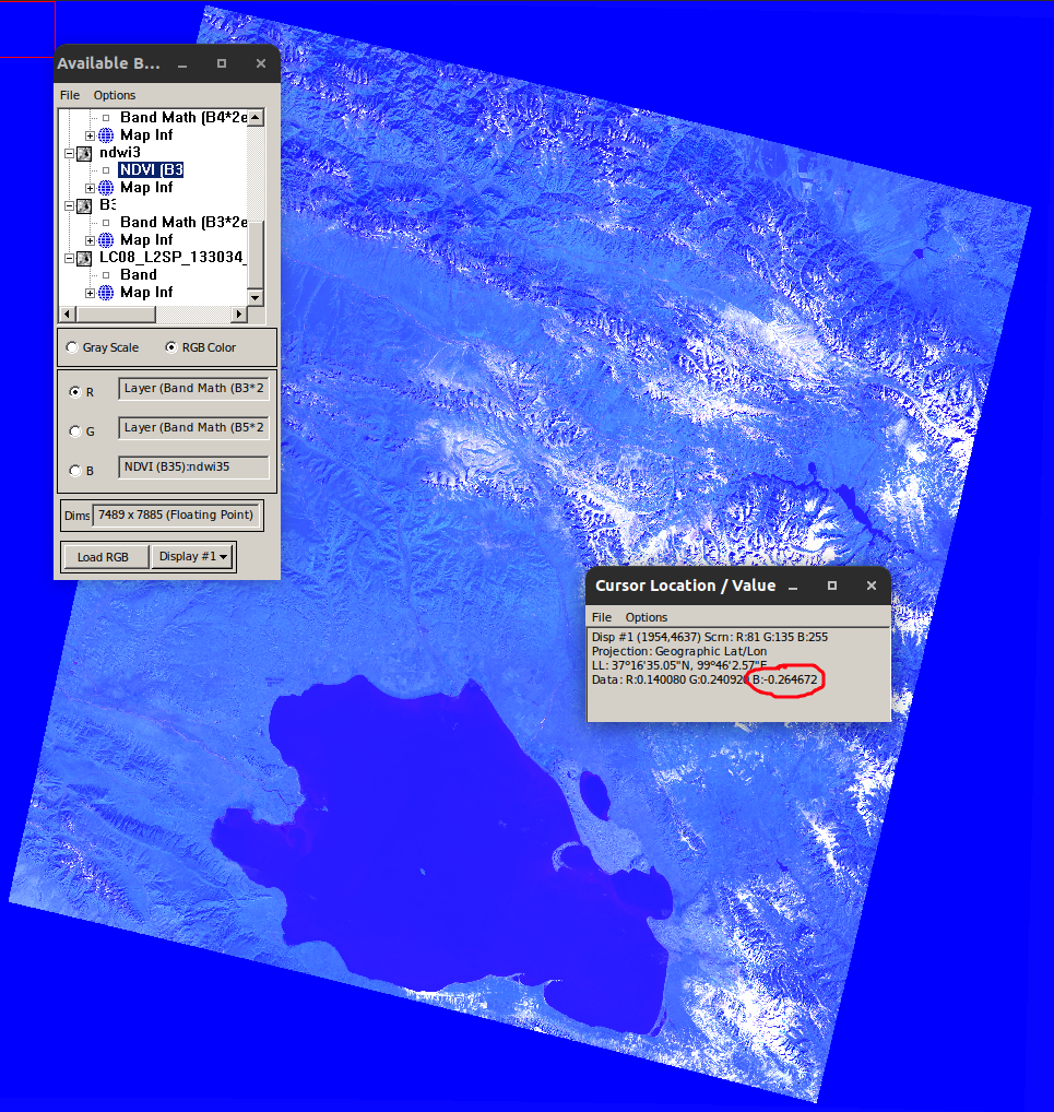
The cursor is hovering over non-water area so we have negative NDWI value

And now we’re almost done with the processes using ENVI! For further processing in MATLAB, we need to convert the map projection from UTM to Geographic Lat/Lon, using Map| Convert Map Projection, and then save the file as TIFF/GeoTIFF.

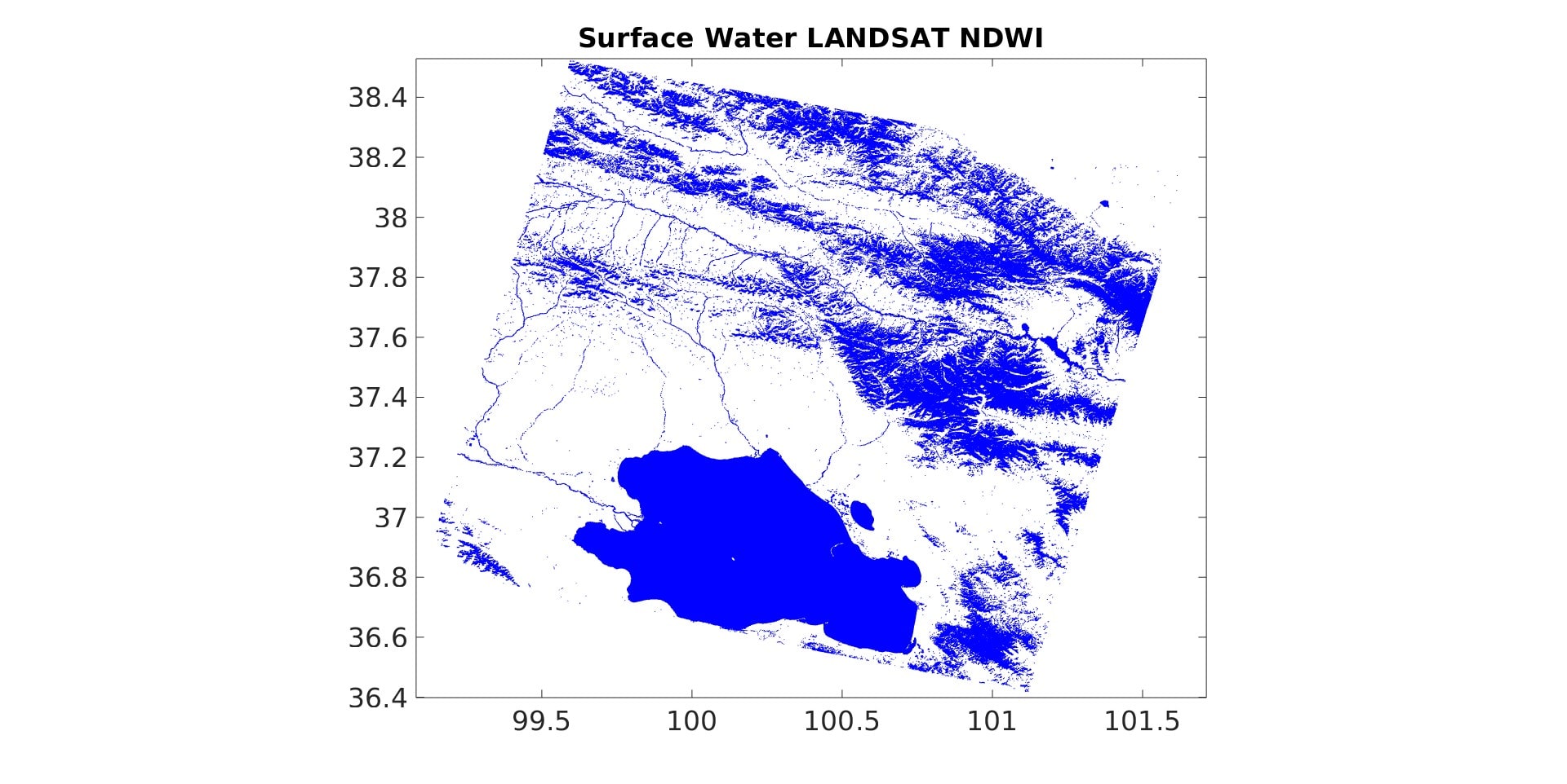
I will write another post for detailed explanation on the MATLAB scripts for extracting water bodies from the NDWI image obtained, and also removing cloud-covered pixels using the BQA file.